


Trong một số trường hợp, thuật toán học máy không cần xem xét toàn bộ tập mẫu học mà vẫn cho ra kết quả hàm phân lớp giống như khi thuật toán chạy trên toàn bộ tập mẫu học. Ví dụ, trong trường hợp perceptron, các mẫu học được sử dụng là các mẫu học bị phân lớp sai trong quá trình học. Trong trường hợp máy học sử dụng véc tơ hỗ trợ (SVM), các mẫu học cần thiết là các véctơ hỗ trợ. Trong bài này, ta sẽ đánh giá độ chính xác của các thuật toán học như vậy.
Để cho tiện, xét tập mẫu học 

![\displaystyle [n] = \{1,\ldots,n\}](https://s0.wp.com/latex.php?latex=%5Cdisplaystyle+%5Bn%5D+%3D+%5C%7B1%2C%5Cldots%2Cn%5C%7D&bg=fafcff&fg=2a2a2a&s=0&c=20201002)
![\displaystyle I\subset [n]](https://s0.wp.com/latex.php?latex=%5Cdisplaystyle+I%5Csubset+%5Bn%5D&bg=fafcff&fg=2a2a2a&s=0&c=20201002)


![\displaystyle -I = [n]\setminus I](https://s0.wp.com/latex.php?latex=%5Cdisplaystyle+-I+%3D+%5Bn%5D%5Csetminus+I&bg=fafcff&fg=2a2a2a&s=0&c=20201002)

Một thuật toán học 


Định nghĩa (tập mẫu học giản lược): Xét 

Gọi
là rủi ro kì vọng của thuật toán
là rủi ro kì vọng của thuật toán
).
là rủi ro thực nghiệm của hàm
trên tập mẫu học
Ta thấy trong trường hợp Perceptron và SVM, nếu 

Định lý (ước lượng xác suất cho tập mẫu học giản lược – compression bound): Xét trường hợp hàm lỗi bị chặn trong khoảng ![\displaystyle [0,1]](https://s0.wp.com/latex.php?latex=%5Cdisplaystyle+%5B0%2C1%5D&bg=fafcff&fg=2a2a2a&s=0&c=20201002)

Định lý cho thấy nếu tập mẫu học có tập giản lược nhỏ thì rủi ro kì vọng càng nhỏ (theo nghĩa xác suất).
Chứng minh: Ta cần đánh giá xác suất để tồn tại một tập mẫu học 

Quá trình ước lượng như sau: đầu tiên ta ước lượng xác suất với một tập giản lược cụ thể 

Bắt đầu, xét một tập
vì 


Bổ đề: Biến ngẫu nhiên ![\displaystyle X\in [0,1]](https://s0.wp.com/latex.php?latex=%5Cdisplaystyle+X%5Cin+%5B0%2C1%5D&bg=fafcff&fg=2a2a2a&s=0&c=20201002)
![\displaystyle E[X]\geq\epsilon](https://s0.wp.com/latex.php?latex=%5Cdisplaystyle+E%5BX%5D%5Cgeq%5Cepsilon&bg=fafcff&fg=2a2a2a&s=0&c=20201002)

Chứng minh bổ đề: ![\displaystyle \epsilon\leq E[X]=\mathrm{Pr}\left\{X>0\right\}E[X|X>0]\leq \mathrm{Pr}\left\{X>0\right\}](https://s0.wp.com/latex.php?latex=%5Cdisplaystyle+%5Cepsilon%5Cleq+E%5BX%5D%3D%5Cmathrm%7BPr%7D%5Cleft%5C%7BX%3E0%5Cright%5C%7DE%5BX%7CX%3E0%5D%5Cleq+%5Cmathrm%7BPr%7D%5Cleft%5C%7BX%3E0%5Cright%5C%7D&bg=fafcff&fg=2a2a2a&s=0&c=20201002)
Áp dụng bổ đề, ta có ![\displaystyle E[L(f_I(x_i), y_i)]=R(\mathcal{A}(D_I))\geq\epsilon](https://s0.wp.com/latex.php?latex=%5Cdisplaystyle+E%5BL%28f_I%28x_i%29%2C+y_i%29%5D%3DR%28%5Cmathcal%7BA%7D%28D_I%29%29%5Cgeq%5Cepsilon&bg=fafcff&fg=2a2a2a&s=0&c=20201002)

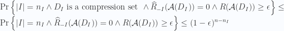
Tiếp tục, dùng ước lượng xác suất tổng, ta có

![\displaystyle \leq \sum_{I\subset [n],|I|=n_I}\mathrm{Pr}\left\{|I| = n_I\wedge D_I \textrm{ is a compression set } \wedge \widehat{R}_{-I}(\mathcal{A}(D_I)) = 0 \wedge R(\mathcal{A}(D_I))\geq\epsilon\right\}](https://s0.wp.com/latex.php?latex=%5Cdisplaystyle+%5Cleq+%5Csum_%7BI%5Csubset+%5Bn%5D%2C%7CI%7C%3Dn_I%7D%5Cmathrm%7BPr%7D%5Cleft%5C%7B%7CI%7C+%3D+n_I%5Cwedge+D_I+%5Ctextrm%7B+is+a+compression+set+%7D+%5Cwedge+%5Cwidehat%7BR%7D_%7B-I%7D%28%5Cmathcal%7BA%7D%28D_I%29%29+%3D+0+%5Cwedge+R%28%5Cmathcal%7BA%7D%28D_I%29%29%5Cgeq%5Cepsilon%5Cright%5C%7D&bg=fafcff&fg=2a2a2a&s=0&c=20201002)
![\displaystyle \leq \sum_{I\subset [n],|I|=n_I} (1-\epsilon)^{n-n_I}](https://s0.wp.com/latex.php?latex=%5Cdisplaystyle+%5Cleq+%5Csum_%7BI%5Csubset+%5Bn%5D%2C%7CI%7C%3Dn_I%7D+%281-%5Cepsilon%29%5E%7Bn-n_I%7D&bg=fafcff&fg=2a2a2a&s=0&c=20201002)


Nếu chọn 

Tiếp tục áp dụng ước lượng xác suất tổng


Ta có điều phải chứng minh.
